Pruning Techniques can be classified as:
- Structured
- For a MLP, structured pruning techniques involves removing an entire feature from a layer. For example, if a layer has size (7,3). Then after pruning the size will be reduced to (5,3).
- Unstructured
- For a MLP, unstructured pruning techniques refers to setting the weights of the individual edge as zero, leading to sparse networks. Unstructured pruning is rather arduous to implement.
We have moved our focus on structured pruning. Structured pruning can be implemented using various techniques namely:
- Iterative
- One-shot.
One-shot
- We first train the model till convergence for a given input number of epochs.
- We begin pruning with certain information in hand such as:
- Pm - pruning ratio which means we will prune pm percent of the features in each layer.
- Trained model - the sequential model post training
- Input size - No of input to the first layer
- Output size - No of output in the last layer. We don’t want to prune this.
- We start off with a for loop that iterates over each layer.
- Let’s say the first layer size is (10,3). It means that there are 10 output and 3 input edges. We find the L1 norm of each column and sort all the 10 layers. Then we remove pm percent of columns that have lowest weights and store that column index information in an array - pruned_layers. Let’s assume 2 features were removed. So instead of 10, there will be only 8 outgoing edges.
- For the next layer, let’s say the size is (14,10). Which means it has 10 input and 14 outgoing edges. Before pruning these layers, we have to remove certain rows from the matrix. This is because in the previous layer certain features were removed - 2 features. So we will remove those rows and repeat the step of finding the L1 norm for each column. Again we will remove pm percent of columns that have lowest weights and store that column index information in an array - pruned_layers.
- We will skip the activation layers in between and repeat the above method till we reach the last layer. We don’t prune the last layer because we have a classification model.
- We return a sequential model re-initialised with random values.
One-shot Reinitialize:
- The above steps are same for the one-shot pruning with a minor modification
- We store the unpruned_layers at each index in an array. Suppose for a layer of size (10,3) we prune 2 features. Then we store the indexing of 8 features in an array. We push the array in a 2d array - unpruned_layers.
- When we finish pruning, we return a sequential model re-initialised with values of the pre-training model.
Iterative Pruning
- The inputs defined for the iterative pruning are
- Max_iter - It defines the number of iterations or epochs we will train the model.
- Prune_iter - It defines the number of iterations in which we will prune. Let’s say we have to prune pm percent in total and there are prune_iter iterations. In each iteration will prune per_round_prune_ratio in each layer.
- We will run a for loop that runs for max_iter number of iterations.
- Inside the for loop whenever we are on the Max_iter/Prune_iter iteration, we will do pruning with a constant pruning ratio = per_round_prune_ratio.
- Pruning analogy here is same as that for one-shot pruning, except here we re-initialize the model with the values of post-training or we can say reinitialize the model with the same values.
- This training and pruning steps repeat till we are done pruning prun_iter no of times.
One important thing to remember in the above method explained for iterative pruning, we are using training as a fine-tuning method, pruning decreases the accuracy. After one-shot pruning we train the model, however after iterative pruning we do not do so.
Results & Observations:
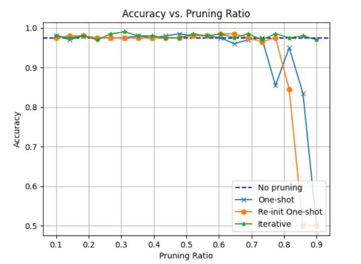
- Iterative Pruning > Re-Init One-shot > One-shot > No-pruning
- Computation is reduced after pruning, which means faster results and more robust relevant features are learned.
- Pruning performance depends on the size of the model. For large models and simpler datasets, pruning of 0.9 can still increase accuracy

